III. CCD and Dewar
IV. Image Quality Requirements
V. Operations
(a) Standard observing
(b) Apertures
(c) High signal-to-noise
(d) Calibration lamps
(e) Long slit
(f) Un-cross-dispersed
(g) High stability
(h) Summary of Operations Requirements
XI. Estimated Cost
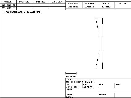
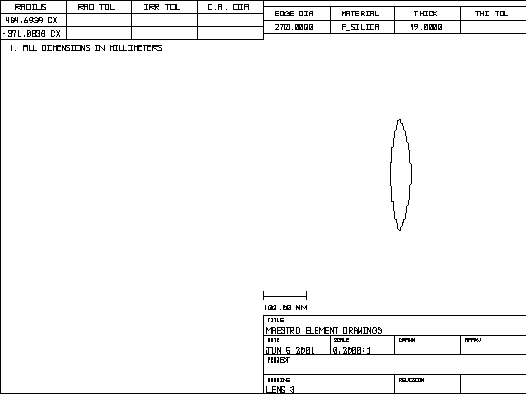
Appendix I: Drawings of individual optical elements
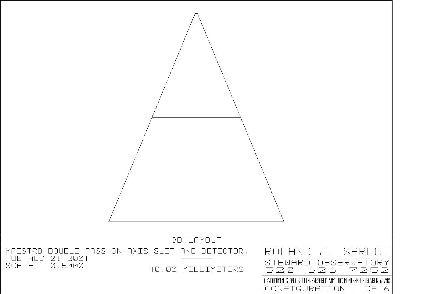
The earlier design located the spectrograph at a Naysmyth platform, using the f/15 secondary. The Naysmyth platform would have to be built, and the optics which directs the beam to the Naysmyth would have to be fabricated. The acquisition/guider camera would have to be made, as well as calibration lamp functions. By placing the spectrograph at f/9 Cassegrain, we can use the existing secondary mirror, "Top Box" and rotator. The target acquisition and guiding scheme will be the same as that used with the MMT spectrographs). Foltz said that this is a preferable solution from the standpoint of operations, despite the fact that the spectrograph would be removed from the telescope when not in use. One potential disadvantage of the Cass location is that the physical size of the spectrograph is limited; however the adopted Litrow design is compact and well within the weight and size limits. A description of the MMT optics is given by Fabricant, McLeod and West.
The plan is to reloctate MAESTRO to LBT at some point. The other planned echelles for the LBT are optimized to be fed by AO (e.g. AVES), and are near-IR or at least red-optimized. Details of the mechanical coupling to the telescope, guiding, calibration etc would be worked out later, and would depend on what has been provided by MODS.
The advantage of a prism cross-disperser is that you can have single exposure coverage which covers more than a factor of 2 in wavelength. For a grating cross-disperser, you are limited to a factor of 2 in wavelength coverage or else you suffer order overlap. By having a very large single-exposure spectral coverage, you can have a point-and-shoot instrument with few moving parts, a very important advantage. A prism is superior in throughput, and spaces the orders more compactly on the detector than a grating.
The disadvantage of a prism is that order separation in the red is poor, just where the sky is bright and sky subtraction is difficult. We therefore will fabricate two sets of prisms, which will be interchangeable. One set will be optimized for the blue, and be transmissive to the atmospheric cut-off. The other will be made of a higher index flint and therefore have better order separation in the red, but not be blue transmissive.
A two channel system offers many advantages, including optimization of the optical design, materials and coatings, over a shorter wavelength range. However, the added complexity of having to fabricate channels, and the unattractive dichroic in the middle of the most sensitive part of the optical spectral range, made us chose a one-channel system with a prism cross-disperser.
There are two science applications we foresee with competing requirements, one (quasars) which requires coverage to the atmospheric cut-off at 320 nm, and the other (stars) which typically requires spectra to the silicon cut-off out at 0.9-1.0 microns. We chose to optimize for the blue, but do not want to preclude the red. Future spectrographs at the LBT will be optimized for use with AO, and should be designed to work to the short wavelength cut-off of InSb. For InSb and red-optimized spectra, the observing sequence is sufficiently different from the optical/CCD observing sequence, that it is not clear that a spectrograph with both near-IR and optical capabilities is desirable. The wavelength coverage is discussed further below.
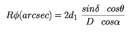
here R = spectral resolution = lambda / ![]()
![]() =
the blaze angle of the echelle grating
=
the blaze angle of the echelle grating
![]() = the angle
of the incident beam onto the grating with respect to the blaze
= the angle
of the incident beam onto the grating with respect to the blaze
![]() =
= ![]() +
+ ![]()
D = the diameter
of the telescope
d1= the
size of the collimated beam at the echelle grating.
Given the beam size of 200 mm and the MMT or LBT telescope primary, and assuming a Littrow configuration, the spectral resolution depends on the blaze angle only.
For the MMT,
R![]() (arcsec)
= 12,683 tan
(arcsec)
= 12,683 tan![]()
and for the LBT,
R![]() (arcsec)
= 9812 tan
(arcsec)
= 9812 tan![]()
We'd like R=30,000 (10 km/sec) at the MMT with a 1 arcsec
slit, so ![]() =67
degrees. With this grating at the LBT, the 1 arcsec resolution is 13 km/sec,
with a 0.7 arcsec slit 9 km/sec. The maximum resolution with 2 pixel sampling
is 3 km/sec, which would require a 0.3 arcsec slit at the MMT or a 0.25
arcsec slit at the LBT.
=67
degrees. With this grating at the LBT, the 1 arcsec resolution is 13 km/sec,
with a 0.7 arcsec slit 9 km/sec. The maximum resolution with 2 pixel sampling
is 3 km/sec, which would require a 0.3 arcsec slit at the MMT or a 0.25
arcsec slit at the LBT.
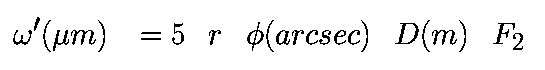
The projected slit width at the detector, ![]() , in microns is
, in microns is
where
r = the anamorphic demagnification
F2 = the camera focal ratio.
In order to get a reasonable plate scale given our 15 micron pixels, we take F2 = 3. In other words, a lens will be needed to take the f/9 or f/15 telescope beam and make it f/3. We assume r=1.0.
Then the scale is 0.154 arcsec/pixel at the MMT and
0.119
arcsec/pixel at the LBT. In order to get a plate scale better
matched to our detector, we'd need a faster camera, which would
be hard to fabricate.
The groove spacing of the echelle grating determines
the length of each order's free spectral range, L.
See Schroeder's Fig. 13.12.
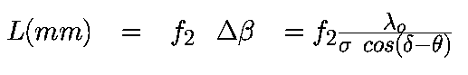
where f 2 =
F2 x 200 mm = 600 mm
![]() =
the distance between grooves
=
the distance between grooves
![]() = the central wavelength of the order.
= the central wavelength of the order.
![]() =
blaze angle of the echelle grating.
=
blaze angle of the echelle grating.
Let Ax be the angular dispersion of the
cross-disperser, in arcsec/length, then
![]() = 2 f2
Ax
= 2 f2
Ax ![]()
where ![]() = the distance between orders in length units
= the distance between orders in length units
f2 = 600 mm
![]() = the free spectral range
= the free spectral range
and the factor of 2 comes from the fact that we use the prism in double pass.
For a prism,

where
t = base length of prism
a = height of the prism
and
![]()
and
![]()
for UBK7. For a 50 degree apex
angle, t/a=0.933.
We settled on a grating blazed at 63 degrees with 79 grooves/mm. The results are summarized in the table below and given in detail in Appendix 2.
In all cases we have continuous spectral coverage blueward of about 650nm, and gaps redward of that.
The optical design described below was carried out
by Sarlot, and assumed a single grating of UBK7
and a 50 degree apex angle. These give acceptable
formats, but with pretty small slits -- we'd have to count on crash hot
image quality.
We then thought about 2 prism systems, with two 35 degree
apex angle prisms. These give
better order separation.
The problem is that UV transmissive glasses like UBK7 have low indices of refraction.
Another possibility is to have two sets of prisms:
- one set is as blue transmissive as possible
- higher index glass to be used only at
wavelengths longward of 400 nm
Once we chose to shorten the single exposure spectral coverage one has to ask if we are not better off with a grating cross-disperser and a more traditional design. The two-prism options cover a little more than a factor of 2 in wavelength, but not much -- first order grating cross-dispersers are limited to a factor of 2 in wavelength. However, a grating cross-disperser has less uniform spacing of orders, so we would not be able to fit the full factor of 2 wavelength coverage on a 4k ccd. Also, even with effectively 8 surfaces, the throughput of the prism cross-disperser is better than a grating.
Thus, we like the 2 prism designs, which will allow red
spectroscopy. A set of red prisms could be made later if they are
not within the current budget.
| Cross disperser | Telescope | Single Exposure Total Wavelength Coverage | Slit Length |
| Single UBK7 50 deg | MMT | 310 - 1000 nm | 7 arcsec |
| Single UBK7 50 deg | LBT | 310 - 1000 nm | 6 arcsec |
| Two 35 deg prisms UBK7 | MMT | 310-700 nm | 10 arcsec |
| Two 35 deg prisms Flint | MMT | 400-900 nm | 12 arcsec |
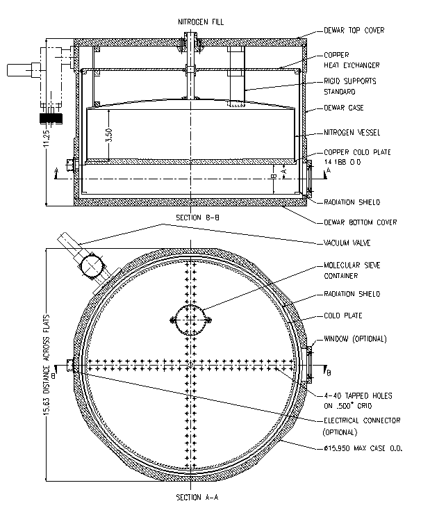
The dewar will be a standard LNe dewar from Infrared Labs, CD-ND-14.
Here we show the QE curve of
the CCD and the atmospheric transmission in the blue, in order to see where
to set the blue limit. We
set 330 nm as the bluest wavelength we optimize in the optical design,
although
we allow work to 310 nm.
The quantum efficiency (QE)
curve for the MAESTRO CCD will be simillar to CCD24 at the 90inch, shown
here.

Although the CCD has high QE all the way down to 0.3200 microns, atmospheric transmission is poor below 0.3400 microns. Some optical image degradation by the spectrograph is tolerable in the blue -- the telescope itself will probably provide further degradation.


Most of the seeing measurements were better than 1 arcsec, and they never measured seeing better that 0.4 arcsec. At the blue end of MAESTRO, we expect the image quality delivered at the slit to be somewhat worse than the seeing measured with the seeing monitor.
The median seeing of 0.8 arcsec FWHM corresponds to a gaussian with
![]() =
0.8 arcsec / 2.354 = 0.34 arcsec.
=
0.8 arcsec / 2.354 = 0.34 arcsec.
Most of the light is within +/2![]() ,
or 1.36 arcsec.
,
or 1.36 arcsec.
The range of the seeing, 0.4 - 1.0 arcsec FWHM, corresponds
to ![]() = 0.17
- 0.425 arcsec, and +/2
= 0.17
- 0.425 arcsec, and +/2![]() =0.7-1.7
arcsec, which 4.7-11 pixels at the MMT. Thus the spectrum will be oversampled
with 15 micron pixels.
=0.7-1.7
arcsec, which 4.7-11 pixels at the MMT. Thus the spectrum will be oversampled
with 15 micron pixels.
The median seeing FWZM of 1.36 arcsec corresponds to
9 pixels at the MMT, and so we'd always bin the CCD down to get 2-3 pixels
per resolution element. If we have optics which can deliver images that
are good enough to allow the observer to have 2.5 pixel sampling with the
15micron pixels and no binning (i.e. have the maximum spectral resolution),
then the full 2![]() gaussian
corresponds to 0.385 arcsec or a FWHM of 0.227 arcsec.
gaussian
corresponds to 0.385 arcsec or a FWHM of 0.227 arcsec.
Guiding and acquisition will
be accomplished with the existing Topbox, which will view the slit.
The slit is tilted 12.5 degrees
with respect to the telescope axis, and the focal plane is 9.0 inches behind
the top box mounting plate.
The current guider has two magnification lenses.
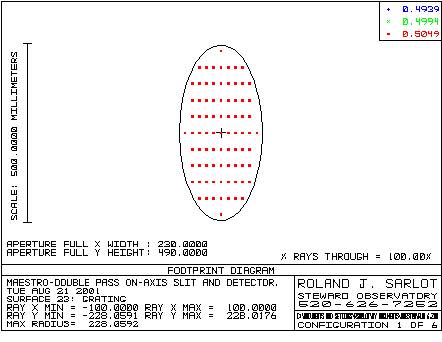
The slit will be machined into an aperture plate, which is then polished and aluminized. The aperture plate will be mounted in a holder which is removable by the observer with the telescope at stow.
The choice of aperture plates will include:
double
small holes for testing and focus
0.7
arcsec x 10 arcsec for standard blue observing
0.7
arcsec x 12 arcsec for standard red observing
1.0
arcsec x 10 arcsec for blue observing during poor weather
1.0
arcsec x 12 arcsec for red observing
0.3
arcsec x 10 arcsec for high spectral resolution
collection of 1 arcmin slits for long slit mode
Small dither motions of the spectrum on the detector, 15-50 microns, will be done by moving the echelle grating.
(f)
Summary of Operational Requirements
Focal ratio at detector: f/3 (for 6 pixels/arcsec or 0.154arcsec/pixel)
Pupil diameter at grating: 200mm
Detector size: 4k x 4k with 15um pixels
Interchangeable between MMT and LBT (with interchangeable focal reducers)
Ability to remove prism and reposition grating
Spectral region: 0.330um to 0.7um (minimum)
Spectral region: 0.310um to 0.85um (optimal)
Prism: Ohara FSL5Y with 50 degree apex angle
Grating: 62 degrees blaze angle, 79 grooves per mm
Slit length: 7 arcseconds long on sky
Imagery: 0.25 to 0.50 arcseconds rms
The design consists of six powered elements and an additional focal changer. The lenses are arranged in three groups with various design functions; the triplet is a color corrected collimator, the negative positive pair is a length reducer and the last two lenses reduce aberrations, in particular, field curvature. The overall layout of the design is shown below.
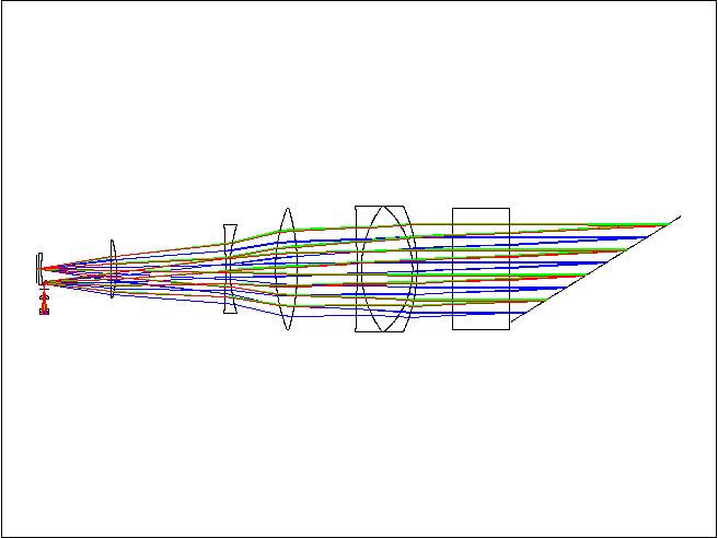
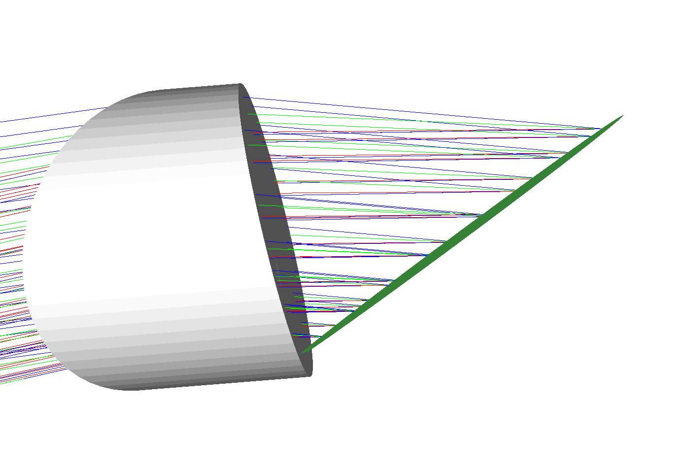
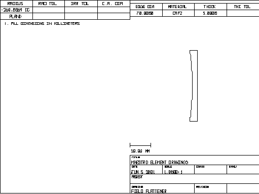
A close-up image of the detector and field flattener is shown below. Note that the small fold flat that reflects the beam after the slit is slightly in front of the detector. However, the shadow of the fold flat is beyond the free spectral range of the data. The image on the right below is viewing the detector from an on-axis ray coming from the grating to the detector. The red color is the full size of the detector, the blue is the shape of the field flattener (it will most likely be cut square later on) and the small ellipse is the fold flat shadow from the mirror after the slit plane.
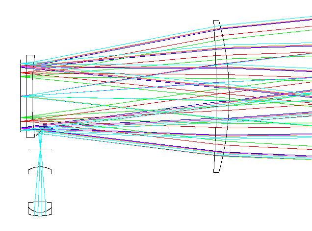
The design corrects color over the spectral region of 0.338um to 0.812um with the model including the telescope, six element lens system and prism with diffraction grating. The focal reducer was modeled with a three lens system before the slit plane, not as the proposed lens/mirror combination. One weakness of this design is that the fold prism reflecting the slit towards the grating is in front of the detector, thus creating a shadow on the detector and losing light. This can be moved either closer to the detector so that the shadow is minimized or angled completely outside of the rays towards the detector which will reduce image quality.
Another
detail that must be finalized is that the bottom of the grating is slightly
touching the prism corner. Moving the grating further away from the prism
deteriorates image quality. Tradeoffs for this may be to allow minimal
vignetting at the bottom of the grating and cut the grating shorter.
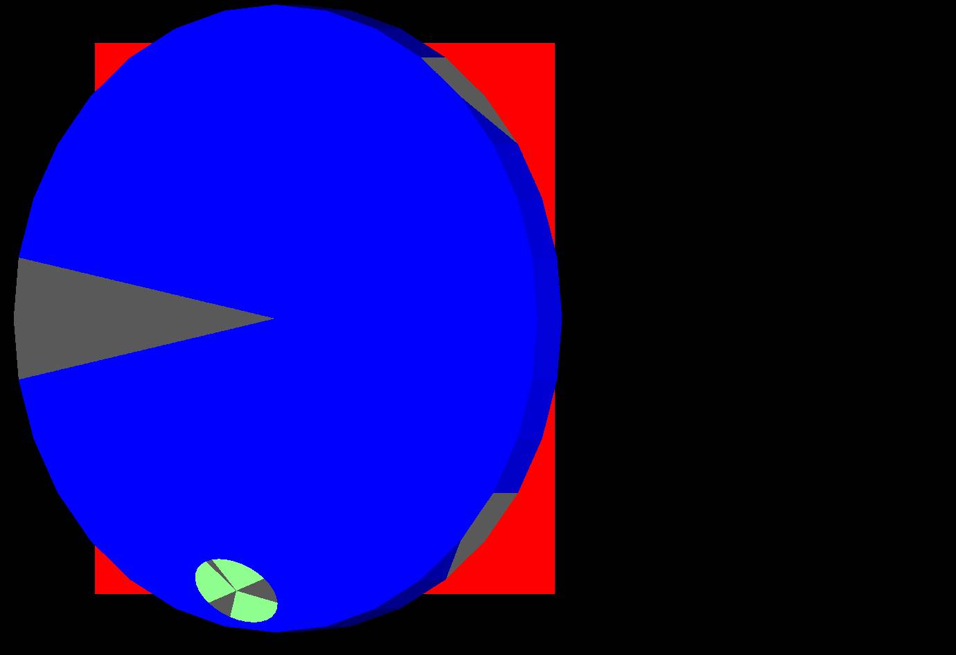
The focal reducer assembly causes a small shadow, shown below.
The red square is the detector, and
the green and grey circle is the shadow of the focal reducer/prism
assembly.
The instrument
will be used on the MMT as well as the LBT with focal ratios f/9 and f/15,
respectively. Therefore Maestro must include a set of focal reducers to
change either incoming beam to an instrument f/3 beam. Originally, a small
three lens set was designed for this purpose that was positioned before
the slit. However, this presented numerous problems, mostly with the external
field viewing camera, and we have now decided to use a combination fold
flat lens. At this time, only initial design work has been carried out
with this technique but the idea looks very promising. Below is a drawing
of the f/9 to f/3 dual purpose fold flat and focal changer immediately
after the slit plane.
The following
performance estimates include the nominal system with a telescope but do
not simulate the atmosphere nor include manufacturing nor alignment errors.
In general, the performance is not yet good enough for manufacturing but
we believe the overall design should not be changed. Instead, the design
needs to be further optimized or perhaps, an additional lens can be added.
The first illustration details the spectra on the detector by order with
longest wavelength on the left and the shortest on the right. The second
image is a representation of the detector with various positions giving
the image quality in arcseconds of the wavelength/order combo of the first
image. The detector orientation is the same as the earlier detector illustration.
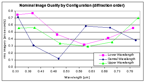
The given specifications were for better than 0.5 arcseconds rms.

Another
method of assessing the performance is looking across the orders. The instrument
was modeled with various multi-configurations representing the order/wavelength
combos from order 28 to 66 with three wavelengths for each order. The following
graph shows the three wavelengths for each order modeled (when three points
are vertically aligned.) The graph depicts imagery for each wavelength
and shows imagery as compared to the specification. In this manner, a reoptimization
can be performed with new weighting to improve the balance over the spectral
region for more consistent performance.
The majority
of the materials are manufactured by Ohara in their I-line series and all
materials are within present volume capabilities of the manufacturer (with
an approximate six month lead time.) The material thickness and transmission
data are given below for various wavelength and is therefore the minimum
transmission for the design at any longer wavelength and field position.
The calculations consider only bulk transmission losses and further light
loss is expected from Fresnel losses, grating efficiency, focal reducer,
the detector efficiency, etc.
|
Material
(inc. double pass)
|
|
@ 0.33um |
@ 0.34um |
@ 0.50um |
|
FPL51Y
|
|
|
|
|
|
BSL7Y
|
|
|
|
|
|
Fused Silica
|
|
|
|
|
|
BSL7Y
|
|
|
|
|
|
CaF2
|
|
|
|
|
|
BAL35Y
|
|
|
|
|
|
FSLFY
|
|
|
|
|
|
BAL35Y
|
|
|
|
|
|
Full transmission
through lenses
|
|
|
|
|
The echelle grating will be from the Richardson
Grating Lab, catalog number 7343LE-401, master BO54.
Richardson Labs has sent information on the reflectance,
based on measurements for a grating made for
CFHT. CFHT has not used the grating in an instrument.
1. The grating is rectangular, and measures 220x420x74
mm.
The ruled area is 204x408
mmxmm.
The groove length is parallel
to the 220 dimension.
2. The substrate is Zerodur.
3. The wavefront specs are lambda/8 rms in the surface, and lambda/2 P-V, where lambda = 330-900 nm.
4. Roland will determine specs for piston, tip-tilt,
both for
initial alignment and for operation.
5. Need to have a motorized micrometer to tip-tilt,
move spectrum
5 pixels at detector, or 60 microns,
in 1 pixel (15micron) steps.
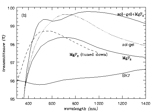
Plain sol-gel is hydroscopic and not sturdy enough for
observatory use. Hardened sol-gel from
Cleveland Coatings is a possibility, but expensive:
90prime had quotes recently of ~$10K per element, for similarly sized pieces.
However, the gain in overall throughput is significant and it is probably worth spending money on coatings.
ZC&R has economical BBAR multilayer coatings, but such coatings are hard to remove if the coating is botched, which has happened.
Tom Ingerson advises that sol-gel + MgF2 is the best choice. He reports measurements of less than 1% reflectance over 330 to 950 nm on witness plates coated with the CTIO ADC optics. The problem is that the only person who has done this type of coating is Jim Stilburn at the DAO, and he is not in the business of coating optics anymore. CTIO has talked about constructing facilities to replicate his technique. We need to seek other sol-gel + MgF2 coating facilities.
With 30 optical surfaces, the transmittance as a function
of coating loss at one surface is given below.
 |
|
Harmer has replaced the triplet with two triplets with thinner elements, and is in the process of optimizing the design.
The field
flattener will be used as the dewar window and we must guarantee that this
element is able to withstand the pressure differential. The aspect ratio
is 14:1. The present window on Aries is 15:1 with the same CaF2 material
and has not yet been tested under a vacuum. We will know the results of
this test within days, nonetheless, many instruments have survived with
similar aspect ratios for the material.
2. Tolerancing needs to be carried out. Sensitivity to alignment and focus need to be quantified.
3. Specs for focus mechanism need to be computed.
4. Specs for grating motion mechanical device need
to be computed.
Diurnal Variations. The observer will focus the spectrograph during the afternoon to adjust for the relatively small changes in focal length from night-to-night temperature variations. The telescope enclosure is kept cooler than the ambient daytime outdoor temperature, since diurnal variations are often large, 20-30 degrees F. The telescope primary thermal control system has been designed to compensate for changes in temperature of 1 degree C per hour (see Fabricant et al for a discussion). We'd like to be able to operate all night without refocusing the spectrograph -- so ideally the focus should not change with changes in temperature of 5 -10 degrees C.
Maximum Variations. The focus mechanism will have to compensate for mechanical expansion and contraction, for the maximum range of temperatures anticipated throughout the year. The telescope thermal system has an operating range of -25 to + 30 degrees C, so this is the range we adopt for the maximum and minimum temperatures of operation.
The large optical elements and detector dewar will be supported on a space frame of carbon fiber poles.
Electronics and other non-critical items will be supported on an outer shell of aluminum.
Preliminary flexure analysis showed that the end-to-end vertical flexure will be approximately 0.0009 inches, or 23 microns, from zenith to horizon. Thus, the innovative use of the space frame promises to exceed performance requirements.


We settled on the 7343LE-401 grating which has a blaze angle of 63 degrees and 79 grooves per mm.
For each choice of cross-disperser and telescope, we compute
R![]() (arcsec) defined above in section
II.c.
(arcsec) defined above in section
II.c.
n = spectral order number
WC(A) = central wavelength of
order in Angstroms
FSR(A) = Free spectral
range in Angstroms
YC(pix) = central pixel
number of each order in the cross-dispersion direction (1-4096 to be on
CCD)
DY(arcsec) = order
separation in arcseconds
(a) Single UBK7 50 degree prism at MMT
Rtheta = 27750.9 (arcsec)
One arcsec maps to 97.5600 microns, or
6.50400 pixels on detector
Order, n WC(A)
FSR(A) FSR(pix) YC(pix)
DY(arcsec):
1 70.
3218. 45.97
2034. 105.
16.1
2 69.
3265. 47.31 2063. 208.
15.9
3 68.
3313. 48.72 2094. 310. 15.6
4 67.
3362. 50.18 2125. 410. 15.4
5 66.
3413. 51.71 2157. 509. 15.2
6 65. 3466.
53.32 2190. 606. 14.9
7 64. 3520. 55.00 2224. 702. 14.7
8 63. 3576. 56.76 2260. 796. 14.5
9 62. 3633. 58.60 2296. 888. 14.3
10 61. 3693. 60.54 2334. 980. 14.0
11 60. 3754. 62.57 2373. 1069. 13.8
12 59. 3818. 64.71 2413. 1158. 13.6
13 58. 3884. 66.96 2455. 1244. 13.3
14 57. 3952. 69.33 2498. 1330. 13.1
15 56. 4023. 71.83 2542. 1414. 12.9
16 55. 4096. 74.47 2588. 1496. 12.6
17 54. 4172. 77.25 2636. 1577. 12.4
18 53. 4250. 80.19 2686. 1656. 12.2
19 52. 4332. 83.31 2738. 1734. 12.0
20 51. 4417. 86.61 2791. 1810. 11.7
21 50. 4505. 90.10 2847. 1885. 11.5
22 49. 4597. 93.82 2905. 1958. 11.3
23 48. 4693. 97.77 2966. 2030. 11.0
24 47. 4793. 101.97 3029. 2100. 10.8
25 46. 4897. 106.46 3095. 2169. 10.6
26 45. 5006. 111.24 3164. 2236. 10.3
27 44. 5120. 116.35 3236. 2302. 10.1
28 43. 5239. 121.83 3311. 2366. 9.9
29 42. 5363. 127.70 3390. 2429. 9.7
30 41. 5494. 134.00 3472. 2490. 9.4
31 40. 5632. 140.79 3559. 2550. 9.2
32 39. 5776. 148.10 3650. 2609. 9.0
33 38. 5928. 156.00 3746. 2665. 8.7
34 37. 6088. 164.54 3848. 2721. 8.5
35 36. 6257. 173.81 3955. 2775. 8.3
36 35. 6436. 183.89 4068. 2827. 8.0
37 34. 6625. 194.86 4187. 2878. 7.8
38 33. 6826. 206.85 4314. 2927. 7.6
39 32. 7039. 219.98 4449. 2975. 7.4
40 31. 7267. 234.40 4592. 3021. 7.1
41 30. 7509. 250.29 4746. 3066. 6.9
42 29. 7768. 267.85 4909. 3110. 6.7
43 28. 8045. 287.32 5084. 3152. 6.4
44 27. 8343. 309.00 5273. 3192. 6.2
45 26. 8664. 333.23 5476. 3231. 6.0
46 25. 9010. 360.42 5695. 3268. 5.7
47 24. 9386. 391.08 5932. 3304. 5.5
48 23. 9794. 425.83 6190. 3339. 5.3
(b)
Single UBK7 50 degree prism at LBT
R![]() =
21443.7
=
21443.7
One arcsec maps to 126.255 microns, or
8.41700 pixels on detector
Order, WC(A), FSR(A), FSR(pix),YC(pix), DY(arcsec):
1 70. 3218. 45.97 2034. 105. 12.4
2 69. 3265. 47.31 2063. 208. 12.3
3 68. 3313. 48.72 2094. 310. 12.1
4 67. 3362. 50.18 2125. 410. 11.9
5 66. 3413. 51.71 2157. 509. 11.7
6 65. 3466. 53.32 2190. 606. 11.6
7 64. 3520. 55.00 2224. 702. 11.4
8 63. 3576. 56.76 2260. 796. 11.2
9 62. 3633. 58.60 2296. 888. 11.0
10 61. 3693. 60.54 2334. 980. 10.8
11 60. 3754. 62.57 2373. 1069. 10.7
12 59. 3818. 64.71 2413. 1158. 10.5
13 58. 3884. 66.96 2455. 1244. 10.3
14 57. 3952. 69.33 2498. 1330. 10.1
15 56. 4023. 71.83 2542. 1414. 10.0
16 55. 4096. 74.47 2588. 1496.
9.8
17 54. 4172. 77.25 2636. 1577.
9.6
18 53. 4250. 80.19 2686. 1656.
9.4
19 52. 4332. 83.31 2738. 1734.
9.2
20 51. 4417. 86.61 2791. 1810.
9.1
21 50. 4505. 90.10 2847. 1885.
8.9
22 49. 4597. 93.82 2905. 1958.
8.7
23 48. 4693. 97.77 2966. 2030.
8.5
24 47. 4793. 101.97 3029. 2100. 8.4
25 46. 4897. 106.46 3095. 2169. 8.2
26 45. 5006. 111.24 3164. 2236. 8.0
27 44. 5120. 116.35 3236. 2302. 7.8
28 43. 5239. 121.83 3311. 2366. 7.6
29 42. 5363. 127.70 3390. 2429. 7.5
30 41. 5494. 134.00 3472. 2490. 7.3
31 40. 5632. 140.79 3559. 2550. 7.1
32 39. 5776. 148.10 3650. 2609. 6.9
33 38. 5928. 156.00 3746. 2665. 6.8
34 37. 6088. 164.54 3848. 2721. 6.6
35 36. 6257. 173.81 3955. 2775. 6.4
36 35. 6436. 183.89 4068. 2827. 6.2
37 34. 6625. 194.86 4187. 2878. 6.0
38 33. 6826. 206.85 4314. 2927. 5.9
39 32. 7039. 219.98 4449. 2975. 5.7
40 31. 7267. 234.40 4592. 3021. 5.5
41 30. 7509. 250.29 4746. 3066. 5.3
42 29. 7768. 267.85 4909. 3110. 5.2
43 28. 8045. 287.32 5084. 3152. 5.0
44 27. 8343. 309.00 5273. 3192. 4.8
45 26. 8664. 333.23 5476. 3231. 4.6
46 25. 9010. 360.42 5695. 3268. 4.4
47 24. 9386. 391.08 5932. 3304. 4.3
48 23. 9794. 425.83 6190. 3339. 4.1
(c) Two 35 degree UBK7 prisms, MMT
Rtheta = 27750.9
One arcsec maps to 97.5600 microns, or
6.50400 pixels on detector
Order, WC(A), FSR(A), FSR(pix),YC(pix), DY(arcsec):
1 70. 3218. 45.97 2034. 147. 22.5
2 69. 3265. 47.31 2063. 291. 22.2
3 68. 3313. 48.72 2094. 433. 21.9
4 67. 3362. 50.18 2125. 574. 21.6
5 66. 3413. 51.71 2157. 712. 21.2
6 65. 3466. 53.32 2190. 848. 20.9
7 64. 3520. 55.00 2224. 982. 20.6
8 63. 3576. 56.76 2260. 1114. 20.3
9 62. 3633. 58.60 2296. 1244. 20.0
10 61. 3693. 60.54 2334. 1372. 19.6
11 60. 3754. 62.57 2373. 1497. 19.3
12 59. 3818. 64.71 2413. 1621. 19.0
13 58. 3884. 66.96 2455. 1742. 18.7
14 57. 3952. 69.33 2498. 1862. 18.4
15 56. 4023. 71.83 2542. 1979. 18.0
16 55. 4096. 74.47 2588. 2094. 17.7
17 54. 4172. 77.25 2636. 2207. 17.4
18 53. 4250. 80.19 2686. 2318. 17.1
19 52. 4332. 83.31 2738. 2427. 16.7
20 51. 4417. 86.61 2791. 2534. 16.4
21 50. 4505. 90.10 2847. 2639. 16.1
22 49. 4597. 93.82 2905. 2741. 15.8
23 48. 4693. 97.77 2966. 2842. 15.5
24 47. 4793. 101.97 3029. 2940. 15.1
25 46. 4897. 106.46 3095. 3036. 14.8
26 45. 5006. 111.24 3164. 3131. 14.5
27 44. 5120. 116.35 3236. 3223. 14.2
28 43. 5239. 121.83 3311. 3313. 13.8
29 42. 5363. 127.70 3390. 3401. 13.5
30 41. 5494. 134.00 3472. 3487. 13.2
31 40. 5632. 140.79 3559. 3570. 12.9
32 39. 5776. 148.10 3650. 3652. 12.6
33 38. 5928. 156.00 3746. 3732. 12.2
34 37. 6088. 164.54 3848. 3809. 11.9
35 36. 6257. 173.81 3955. 3885. 11.6
36 35. 6436. 183.89 4068. 3958. 11.3
37 34. 6625. 194.86 4187. 4029. 10.9
38 33. 6826. 206.85 4314. 4098. 10.6
39 32. 7039. 219.98 4449. 4165. 10.3
40 31. 7267. 234.40 4592. 4230. 10.0
41 30. 7509. 250.29 4746. 4293. 9.7
42 29. 7768. 267.85 4909. 4354. 9.3
43 28. 8045. 287.32 5084. 4412. 9.0
44 27. 8343. 309.00 5273. 4469. 8.7
45 26. 8664. 333.23 5476. 4523. 8.4
46 25. 9010. 360.42 5695. 4576. 8.0
47 24. 9386. 391.08 5932. 4626. 7.7
48 23. 9794. 425.83 6190. 4674. 7.4
(d) Two 35 degree prisms at the MMT, made out of material with 1.2x the index of UBK7
Rtheta = 27750.9
One arcsec maps to 97.5600 microns, or
6.50400 pixels on detector
Order, WC(A), FSR(A), FSR(pix),YC(pix), DY(arcsec):
1 70. 3218. 45.97 2034. 226. 34.8
2 69. 3265. 47.31 2063. 449. 34.3
3 68. 3313. 48.72 2094. 669. 33.8
4 67. 3362. 50.18 2125. 885. 33.3
5 66. 3413. 51.71 2157. 1098. 32.8
6 65. 3466. 53.32 2190. 1309. 32.3
7 64. 3520. 55.00 2224. 1515. 31.8
8 63. 3576. 56.76 2260. 1719. 31.3
9 62. 3633. 58.60 2296. 1919. 30.8
10 61. 3693. 60.54 2334. 2116. 30.3
11 60. 3754. 62.57 2373. 2310. 29.8
12 59. 3818. 64.71 2413. 2501. 29.3
13 58. 3884. 66.96 2455. 2688. 28.8
14 57. 3952. 69.33 2498. 2872. 28.3
15 56. 4023. 71.83 2542. 3053. 27.8
16 55. 4096. 74.47 2588. 3231. 27.3
17 54. 4172. 77.25 2636. 3405. 26.8
18 53. 4250. 80.19 2686. 3577. 26.3
19 52. 4332. 83.31 2738. 3745. 25.8
20 51. 4417. 86.61 2791. 3909. 25.3
21 50. 4505. 90.10 2847. 4071. 24.8
22 49. 4597. 93.82 2905. 4229. 24.3
23 48. 4693. 97.77 2966. 4384. 23.8
24 47. 4793. 101.97 3029. 4536. 23.3
25 46. 4897. 106.46 3095. 4685. 22.9
26 45. 5006. 111.24 3164. 4830. 22.4
27 44. 5120. 116.35 3236. 4972. 21.9
28 43. 5239. 121.83 3311. 5111. 21.4
29 42. 5363. 127.70 3390. 5247. 20.9
30 41. 5494. 134.00 3472. 5379. 20.4
31 40. 5632. 140.79 3559. 5509. 19.9
32 39. 5776. 148.10 3650. 5635. 19.4
33 38. 5928. 156.00 3746. 5757. 18.9
34 37. 6088. 164.54 3848. 5877. 18.4
35 36. 6257. 173.81 3955. 5993. 17.9
36 35. 6436. 183.89 4068. 6106. 17.4
37 34. 6625. 194.86 4187. 6216. 16.9
38 33. 6826. 206.85 4314. 6323. 16.4
39 32. 7039. 219.98 4449. 6426. 15.9
40 31. 7267. 234.40 4592. 6526. 15.4
41 30. 7509. 250.29 4746. 6623. 14.9
42 29. 7768. 267.85 4909. 6717. 14.4
43 28. 8045. 287.32 5084. 6807. 13.9
44 27. 8343. 309.00 5273. 6895. 13.4
45 26. 8664. 333.23 5476. 6979. 12.9
46 25. 9010. 360.42 5695. 7059. 12.4
47 24. 9386. 391.08 5932. 7137. 11.9
48 23. 9794. 425.83 6190. 7211. 11.4

